Using Machine Learning to Forecast Energy in Spain

A high-level view of the forecasting workflow used in this project: combine national power data, weather data, engineered time/solar features, and machine-learning models to benchmark against Spain's day-ahead forecasts for solar and wind power, total load, and price. Image was generated using AI.

 

Why Energy Forecasting Is a Useful Machine-Learning Problem

Energy forecasting is one of those problems where the stakes are immediately practical. If grid operators can predict demand, renewable generation, and electricity prices more accurately, they can schedule supply more efficiently, reduce operating costs, and make better use of variable renewable energy. Solar and wind are especially interesting from a data-science perspective because they are physically driven by weather, time of day, season, and geography - and those relationships are often nonlinear.

 

For this project, we wanted to explore how far we could get using publicly available data and a typical data-science workflow. The goal was not to beat a national transmission system operator with access to plant-level telemetry and purpose-built operational forecasts. Instead, the goal was to build a transparent forecasting pipeline in Python, benchmark it against Spain's 24-hour forecasts, and understand where common machine-learning models succeed and fail.

 

We started with a more traditional time-series baseline using SARIMAX, and then moved to LightGBM, a gradient-boosted decision-tree model. Later in the series, we also bring in satellite-derived solar radiation data from CAMS to see whether better solar features improve the forecast.

 

The Kaggle Spain Energy Dataset

The starting point was the Energy consumption, generation, prices and weather dataset on Kaggle, uploaded by Kolasniwash. We chose this dataset as it contains both power and weather data perfect for building ML forecast models and was easily accessible. The dataset covers four years of hourly data, from 1 January 2015 to 31 December 2018. The power data includes national electricity generation, total load, prices, and day-ahead forecast columns while the weather data contains hourly observations from the OpenWeather API for five large Spanish cities: Madrid, Bilbao, Barcelona, Seville, and Valencia.

 

That combination makes the dataset a great learning tool: it includes both the target variables and a set of weather covariates. It also contains a built-in benchmark, because the solar, wind, load, and price forecast columns can be compared against our own models. The limitation, which becomes important later, is that the weather data is only available for major cities, while much of Spain's solar and wind generation occurs away from those locations.

 

Cleaning and Narrowing the Power Data

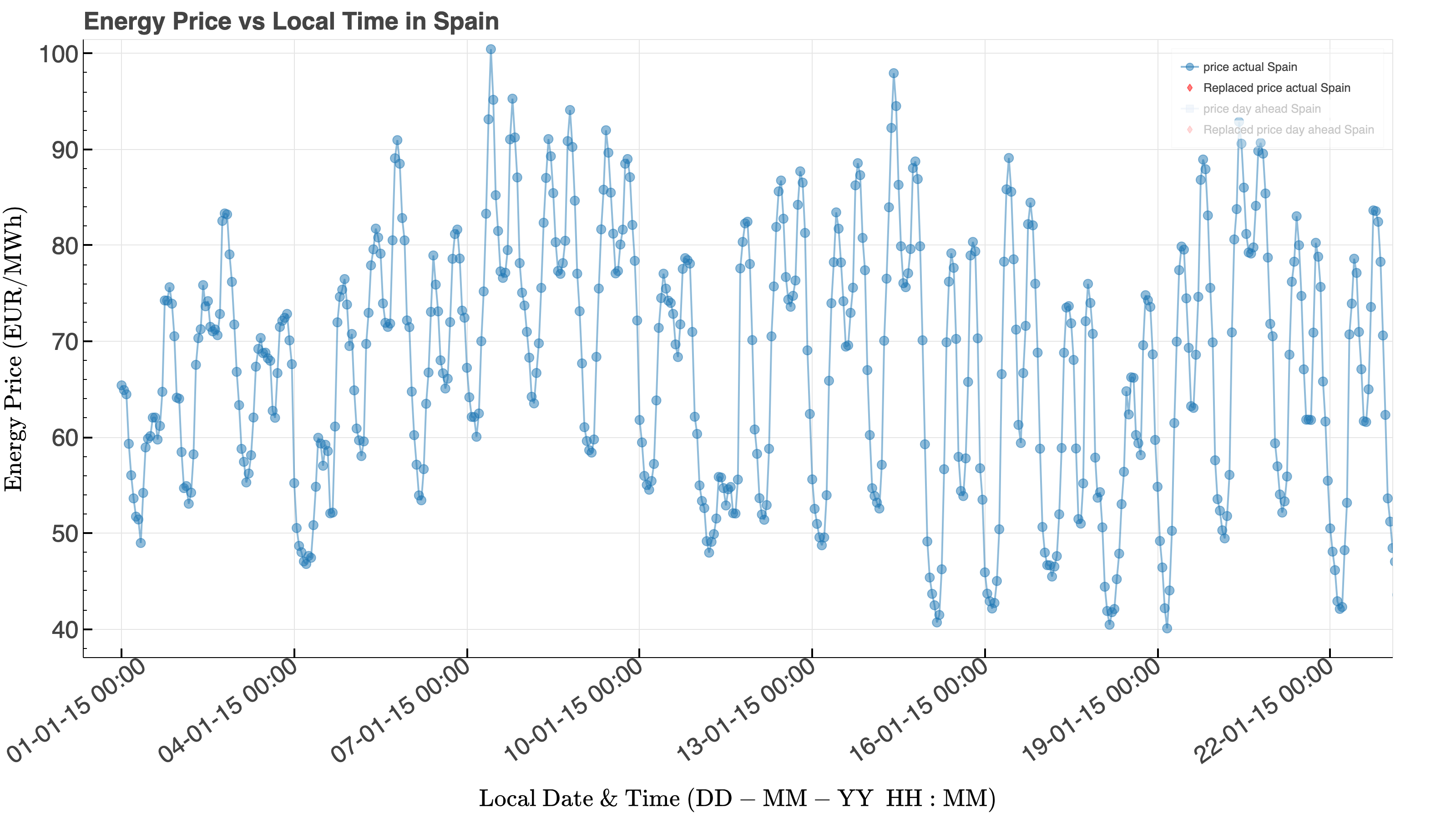
The power table originally contained many generation categories, including biomass, fossil gas, fossil oil, hydro, nuclear, solar, wind, and others. For this project we focused on four targets: solar generation, wind onshore generation, total load, and actual price. We also kept the corresponding day-ahead forecast columns where available, since these provide the benchmark we use throughout the project.

 

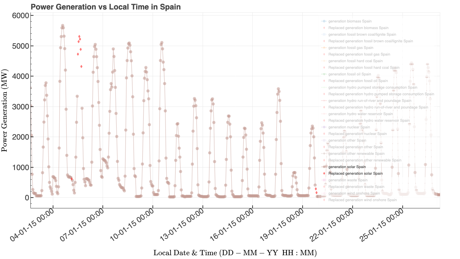
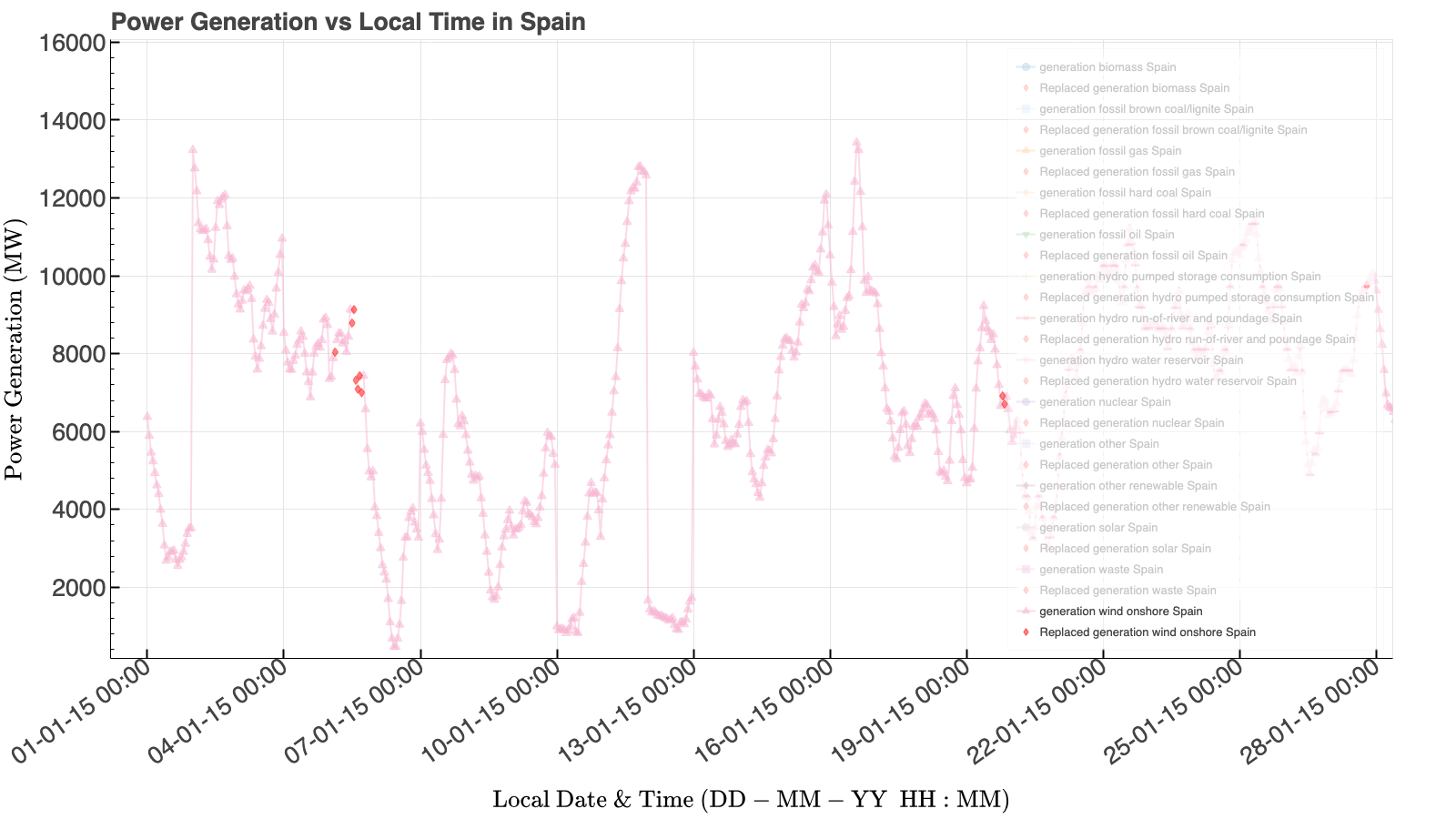
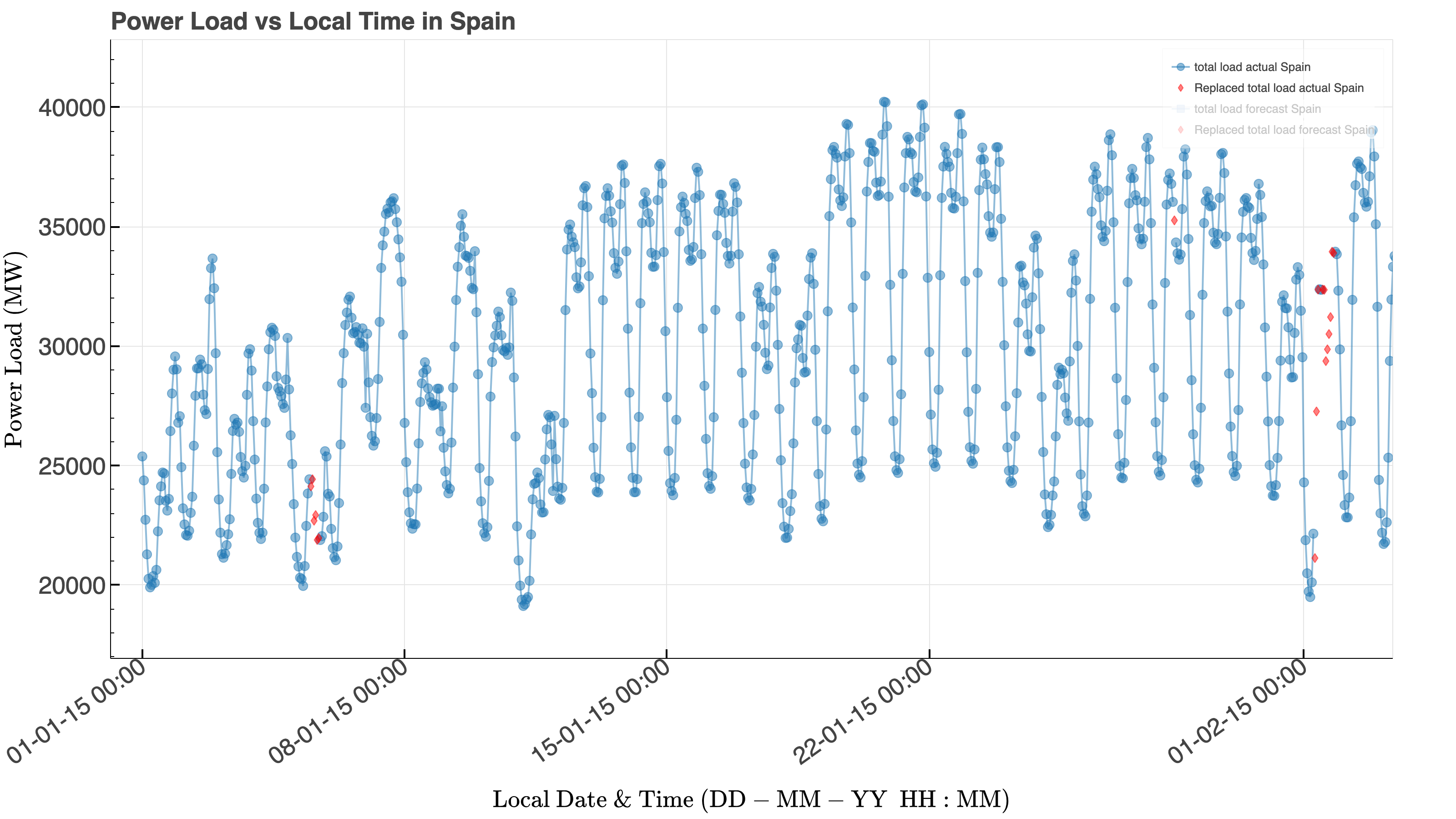
Several of the target columns contained missing values. Solar generation needed special handling because it follows a daily, daylight-driven curve. For short gaps during the day, interpolation was sufficient. For larger gaps, we fitted a local sinusoidal curve using nearby days. Missing nighttime values were replaced with the median value for that night. Wind generation and total load were handled a bit differently, we found using rolling means to replace small gaps and LOESS smoothing, using the loess PyPI library, for larger gaps worked best.

 

Left: Solar generation over a January 2015 interval. The red diamonds mark values imputed during cleaning. Solar is strongly cyclical, but the daytime peaks vary substantially from day to day. Right: Wind generation over January 2015 where the red diamonds mark imputed values. Compared with solar, the wind time series is much less regular, which foreshadows why wind forecasting is harder with this dataset.

 

Left: Total load over a roughly one month period with red diamonds indicating replacements for missing values. Load has a clear daily/weekly rhythm but still changes with weather, season, and holidays. Right: Electricity price over a January 2015 interval. Prices are noisier than load and are influenced by several market and system factors.

 

Cleaning the Weather Data

The weather table contained one row per city per hour, but there were more rows than expected. The excess rows came from duplicate city-time combinations where multiple weather conditions were reported. To handle this consistently, we created a severity score from the OpenWeather condition code. Clear sky received the lowest severity, followed by clouds, mist/fog, drizzle, rain/snow, and thunderstorms. For duplicate entries, we kept the row with the most severe weather condition, breaking ties with the larger weather ID.

 

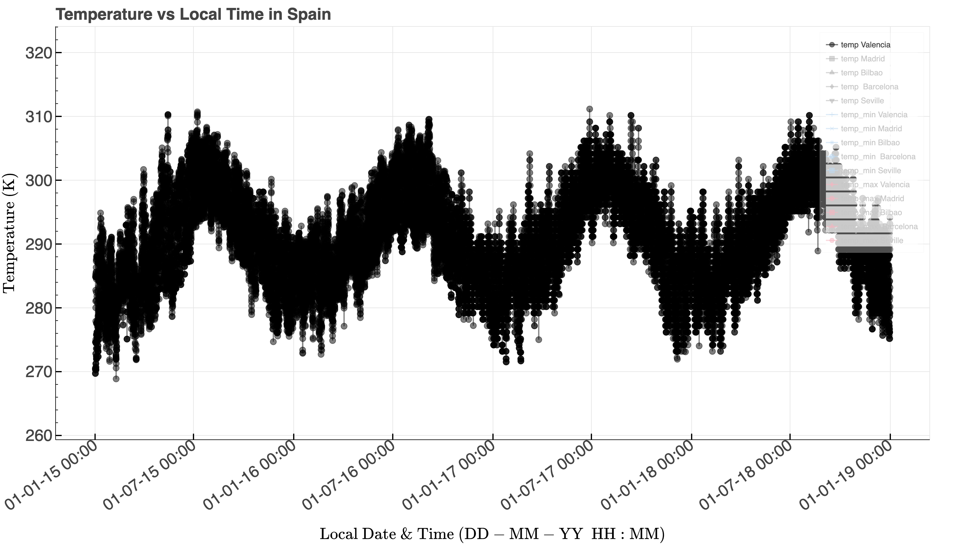
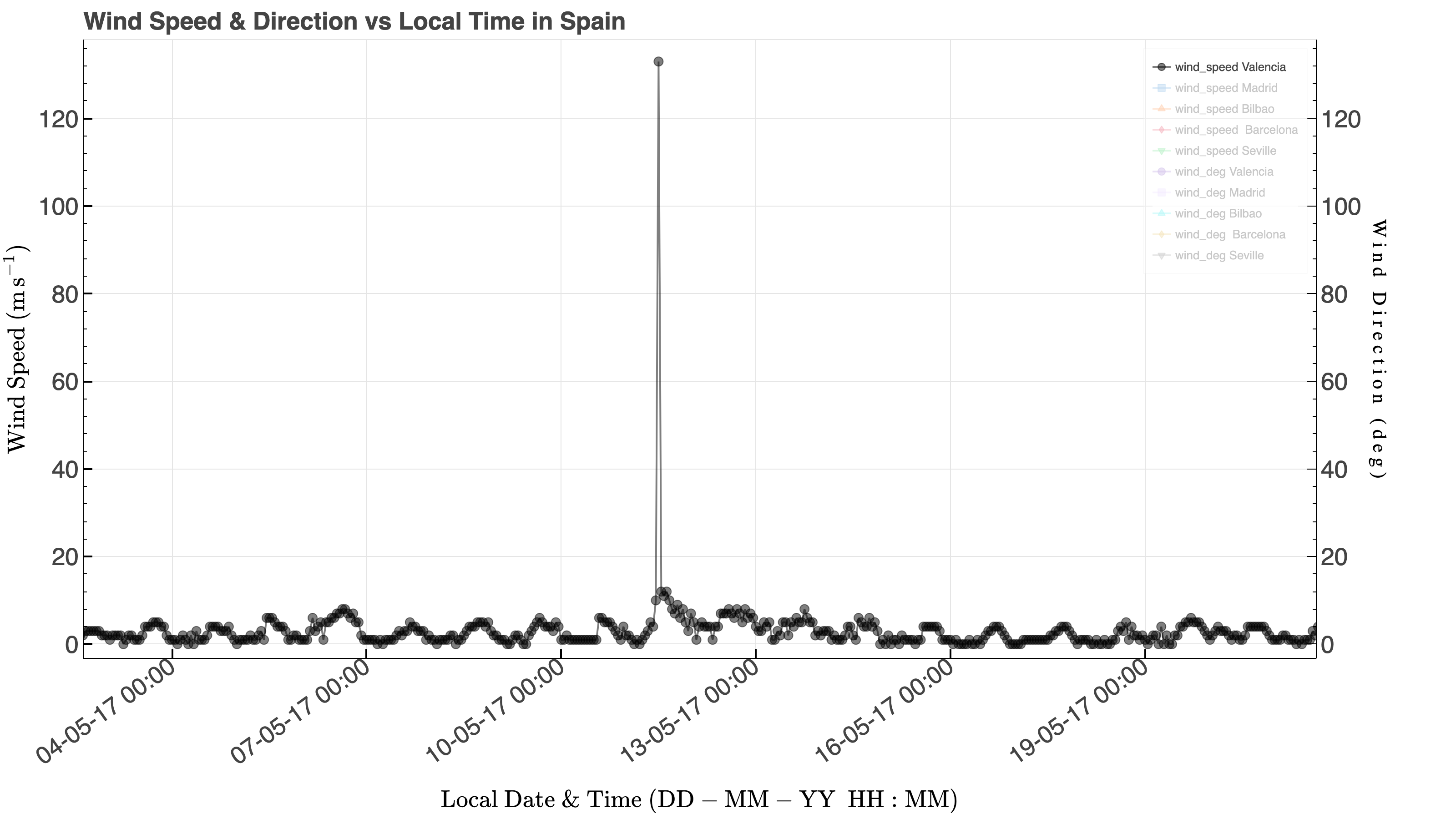
The weather data also contained a few physically implausible values. Pressure values of 0 hPa or enormous values far above any realistic surface pressure were replaced. A wind speed of 133 m/s was also treated as an outlier. We replaced invalid pressure and wind-speed values using rolling medians. For rainfall, we recomputed the 3-hour accumulation from the 1-hour rainfall values because the provided 3-hour column appeared inconsistent.

 

Left: Valencia temperature over the full four-year span. The daily cycle and seasonal cycle are both visible. Right: Valencia wind speed around a clear outlier near 133 m/s. This value was replaced during cleaning.

 

What Comes Next

After cleaning, the weather and power data were merged by UTC time. Because the weather data has five rows per timestamp and the power data has one national row per timestamp, the national power values were broadcast across each city for feature engineering. In the next post, we turn this cleaned dataset into model-ready features and build our first forecasting baseline using ARIMAX.

 

Summary of the skills applied in this work: Python, Pandas, data cleaning, outlier detection, time-series imputation, exploratory visualization, and feature preparation.

 

 

Data Science Home Page ⌂         |         Next Post >