Dr. Brett Addison's Data Science Projects & Blog

Data Scientist | Astrophysicist



Welcome to my data science page, the place where I discuss topics and projects in the field of data science that I am currently working on or have worked on in the past.

Why Add CAMS?
The Kaggle dataset were useful for learning, but it had a major limitation: the weather observations came from only five large cities. That may be reasonable for national load, which is strongly linked to population centres, but it is not ideal for solar and wind generation. Solar plants and wind farms are often far from those cities, and local weather can differ substantially.
To improve solar forecasting, we replaced the Kaggle weather data with data from the Copernicus Atmosphere Monitoring Service (CAMS), accessed through the Atmosphere Data Store. CAMS provides global atmospheric and solar-radiation products, including the CAMS solar radiation time-series. For solar power, the most useful variable is global horizontal irradiation (GHI), which measures solar energy received at ground level and already responds to cloud cover and atmospheric conditions.

Why Try LightGBM?
After the ARIMAX baseline, we moved to LightGBM, a gradient-boosted decision-tree model developed by Microsoft Research. Gradient boosting is well suited to tabular datasets with nonlinear relationships, feature interactions, and heterogeneous inputs. LightGBM is also fast and memory efficient, which mattered because this project was developed on a 2018 MacBook Pro rather than a high-performance compute system.
The first LightGBM models used the same cleaned and engineered Kaggle-derived features as the ARIMAX models: weighted weather features, solar/time features, rolling averages, lags, holiday flags, and cyclical encodings. We trained a mean regression model and also trained quantile models to estimate P16, P50, and P84 predictions, providing a useful 1σ style prediction band.

From Cleaned Data to Model-Ready Features
After cleaning the Spain power and weather data, the next challenge was feature engineering. The targets - solar generation, wind generation, total load, and price - are national values, but the weather observations are city-level measurements. To make the features match the national targets, we aggregated weather features across the five cities using population-based weights. This is a reasonable first-order approximation for load forecasting, although it is less physically appropriate for generation, where the locations of solar plants and wind farms matter much more.
We also added time features that should help the models learn predictable cycles: month, day of year, day of week, weekend flag, public holidays, sunrise and sunset times, daylight length, and cyclical sine/cosine encodings for the hour of day, day of week, day of year, and month. For solar, we also calculated an approximate solar flux using the Sun's position. Rolling and lagged features were added carefully using shifted values so that each row only had access to the past, avoiding data leakage.

Why Energy Forecasting Is a Useful Machine-Learning Problem
Energy forecasting is one of those problems where the stakes are immediately practical. If grid operators can predict demand, renewable generation, and electricity prices more accurately, they can schedule supply more efficiently, reduce operating costs, and make better use of variable renewable energy. Solar and wind are especially interesting from a data-science perspective because they are physically driven by weather, time of day, season, and geography - and those relationships are often nonlinear.
For this project, we wanted to explore how far we could get using publicly available data and a typical data-science workflow. The goal was not to beat a national transmission system operator with access to plant-level telemetry and purpose-built operational forecasts. Instead, the goal was to build a transparent forecasting pipeline in Python, benchmark it against Spain's 24-hour forecasts, and understand where common machine-learning models succeed and fail.
In my previous blog post (see Part 4), I built a random forest classifier model to predict whether orbital obliquities are aligned, misaligned, or highly misaligned. While the model had some success, its performance was limited due to dataset imbalance, where the majority (~60%) of obliquities were aligned, leaving fewer examples for the other two categories (~15% and ~25%, respectively). This small dataset (226 systems) constrained the model's ability to generalize effectively.
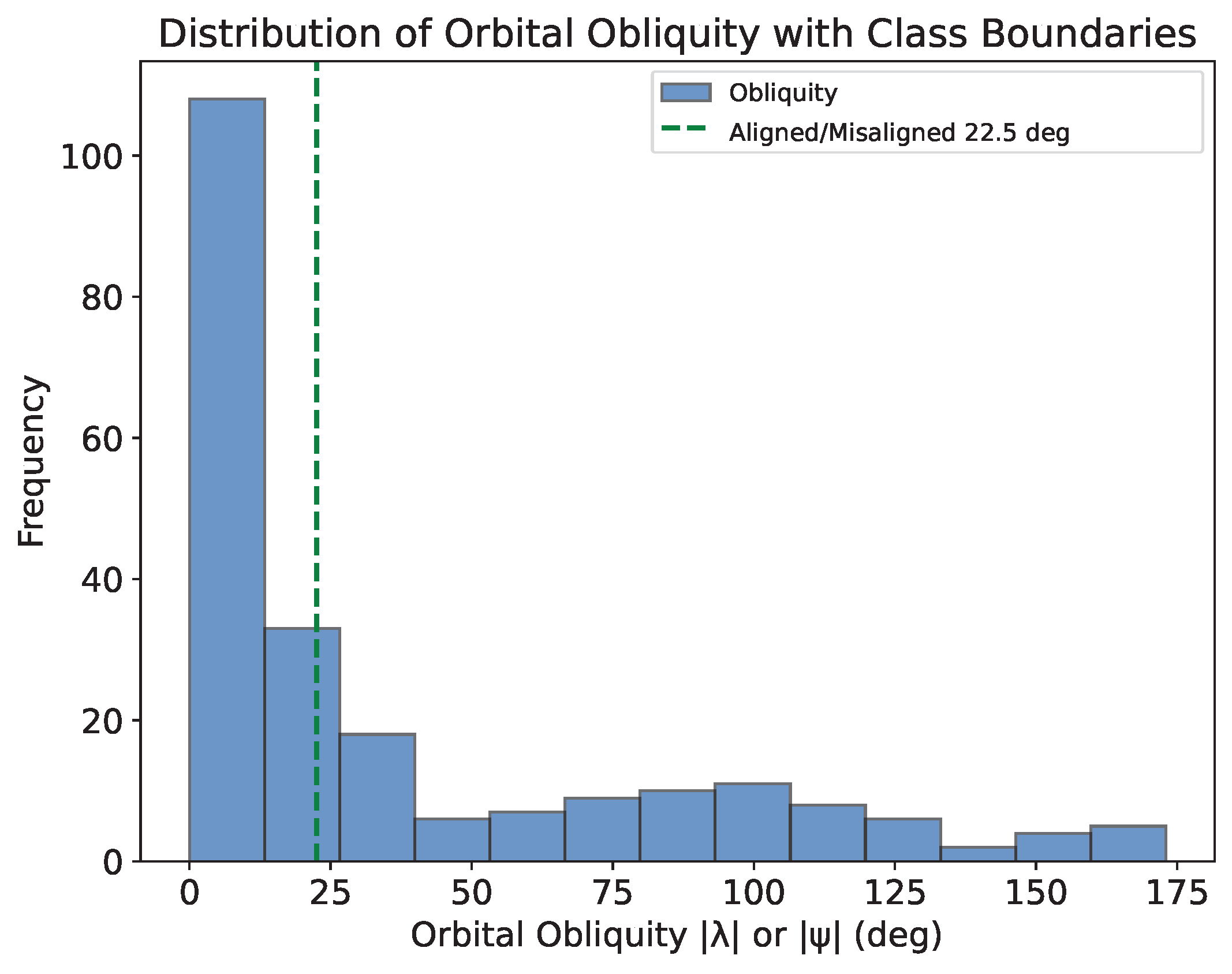
To improve performance, I reduced the classification to just two categories: aligned (λ < π/8 or λ < 22.5°) and misaligned (λ ≥ π/8 or λ ≥ 22.5°). This adjustment created a more balanced dataset (60% aligned, 40% misaligned), compared to the distribution across three categories, as illustrated by the figure at the top of the page, and improved training diversity.
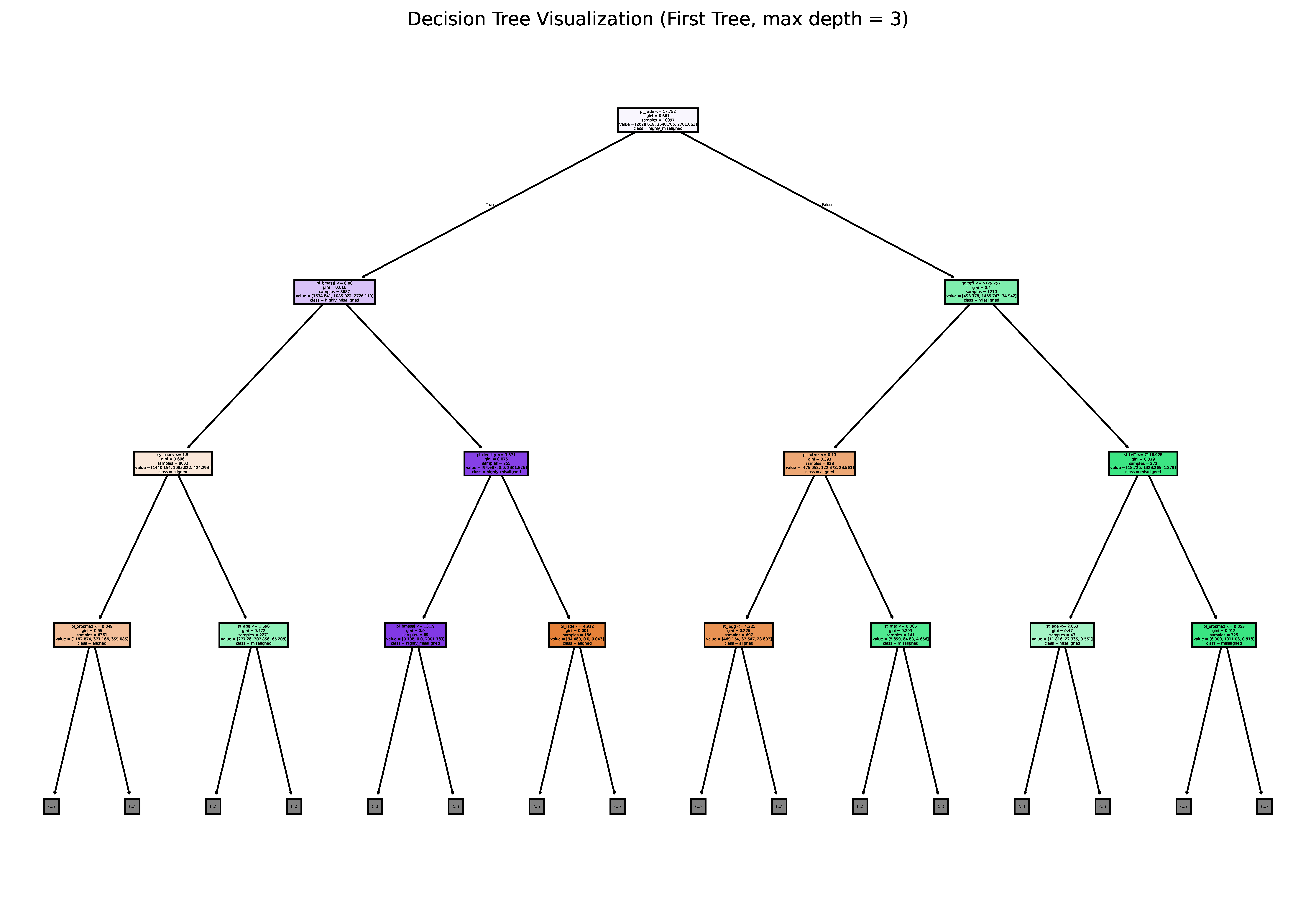
In my previous posts (Parts 2 and 3), I discussed using a random forest regression model to predict exoplanet orbital obliquities based on stellar and planetary parameters. However, its predictive accuracy was limited. In this post, I shift to a classification approach using Scikit-learn's RandomForestClassifier, categorizing obliquities into aligned (λ < 22.5°), misaligned (22.5° ≤ λ < 67.5°), and highly misaligned (λ ≥ 67.5°)—following how they are defined in Addison et al. (2013).
Data Preparation and Feature Engineering
The dataset is compiled using the same preprocessing steps as before, including replacing missing values using physically derived estimates instead of median imputation as well as using the same engineered features—planet-to-star mass ratio (pl_ratmom) and planet density (pl_density), as discussed in Part 3). To account for uncertainties, I again augment the dataset by simulating 100 additional data points per row based on the 1 σ errors.
As discussed in part 2 of this blog series, the current random forest model struggles to predict the orbital obliquities of exoplanets accurately. This may be due to factors such as the small sample size, imbalanced dataset, reliance on median imputation for missing data, insufficiently relevant features, and/or the random forest method being unsuitable for this problem. In part 3, I address these challenges with two enhancements: physically derived imputation and feature engineering.
-
Physically Derived Imputation: Instead of median-based imputation (replacement), missing values are calculated using established relationships between features. For example, the mass of a star can be derived from its effective temperature and radius, assuming it is on the main sequence. This approach produces more accurate and physically meaningful values compared to median replacement.
-
Feature Engineering: Orbital obliquity may depend more on combinations of features than individual ones. To test this, I created two new features: the planet-to-star mass ratio (Mp/M*) and planetary density. These features aim to better capture the dependencies related to obliquity.
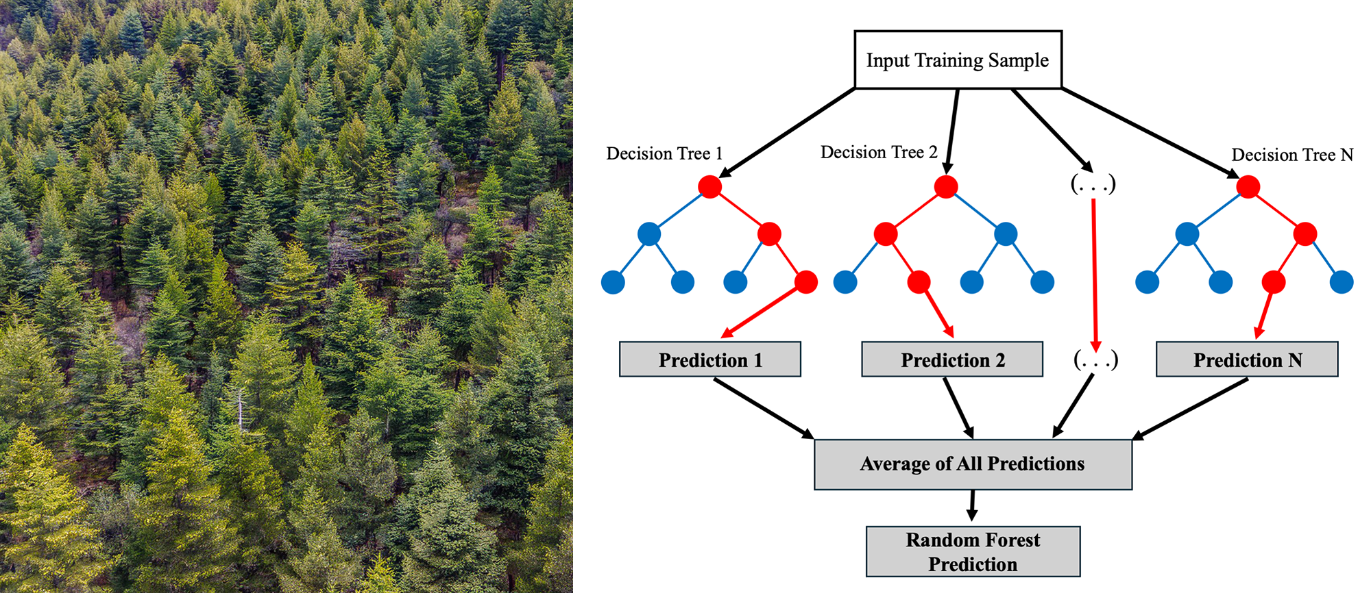
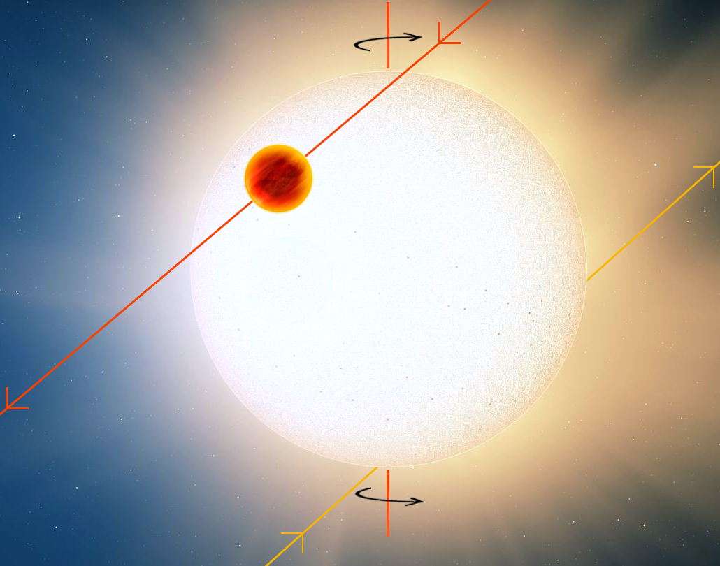
In this project, I applied machine learning to explore an interesting question in astronomy: Can we predict the orbital obliquities of exoplanets using their host stars' properties and planetary system features? Orbital obliquity—the angle between a planet's orbital plane and the equator of its host star—offers crucial insights into planetary formation and evolution. Here's how I approached this challenge using a random forest regression model.
Data Collection and Pre-processing
The first step involved obtaining data from two databases: the catalog of the physical properties of transiting planetary systems (TEPCat) and the NASA Exoplanet Archive. These sources provided the required properties of the exoplanets and their host star's to build a machine learning model, including, for example, the masses, radii, orbital distances, and orbital obliquities. However, the sample size of planets with measured orbital obliquities was small and the measurements came with significant uncertainties. Additionally, the dataset is somewhat imbalanced, there are more than double the number of planets on low obliquity orbits compared to high obliquity orbits as shown in the figure below.
What are Exoplanets?
Extrasolar planets (exoplanets) are planets that orbit stars outside of the Solar System. I have been truly fascinated by the sheer diversity of exoplanets that have been discovered in my field of research over the past three decades. Nearly all of the over 5,000 exoplanets discovered to date look nothing like the planets we have in the Solar System (check out the NASA Exoplanet Archive for the latest tally)! These planets range from scorching "hot Jupiters"--Jupiter-sized planets that whip around their star in only a few days--to super-Earths and mini-Neptunes (planets between the size of Earth and Neptune), and even planets that orbit around their parent star backwards (retrograde). This incredible variety contrasts starkly with the orderly configuration of the Solar System, where planets follow near-coplanar orbits aligned with the Sun's equator.
This raises an intriguing question: Is the Solar System unique?
How Are Exoplanets Detected?
To address this question, I will first cover the two primary methods of discovering exoplanets and their detection biases. These two methods are the transit method and the radial velocity method (see the excellent review of exoplanet detection methods by Jason Wright and Scott Gaudi).