Using Machine Learning to Forecast Energy in Spain

Conceptual overview of the CAMS-based solar forecasting and future-work workflow. Atmospheric and solar-radiation observations are matched to major Spanish solar-plant locations, aggregated using capacity-based weights, and used to generate a national forecast with uncertainty. The southeast Queensland inset represents a future, more geographically aligned project linking local weather observations, renewable-energy assets, load centres, and probabilistic forecasting. Image was generated using AI.

 

Why Add CAMS?

The Kaggle dataset were useful for learning, but it had a major limitation: the weather observations came from only five large cities. That may be reasonable for national load, which is strongly linked to population centres, but it is not ideal for solar and wind generation. Solar plants and wind farms are often far from those cities, and local weather can differ substantially.

 

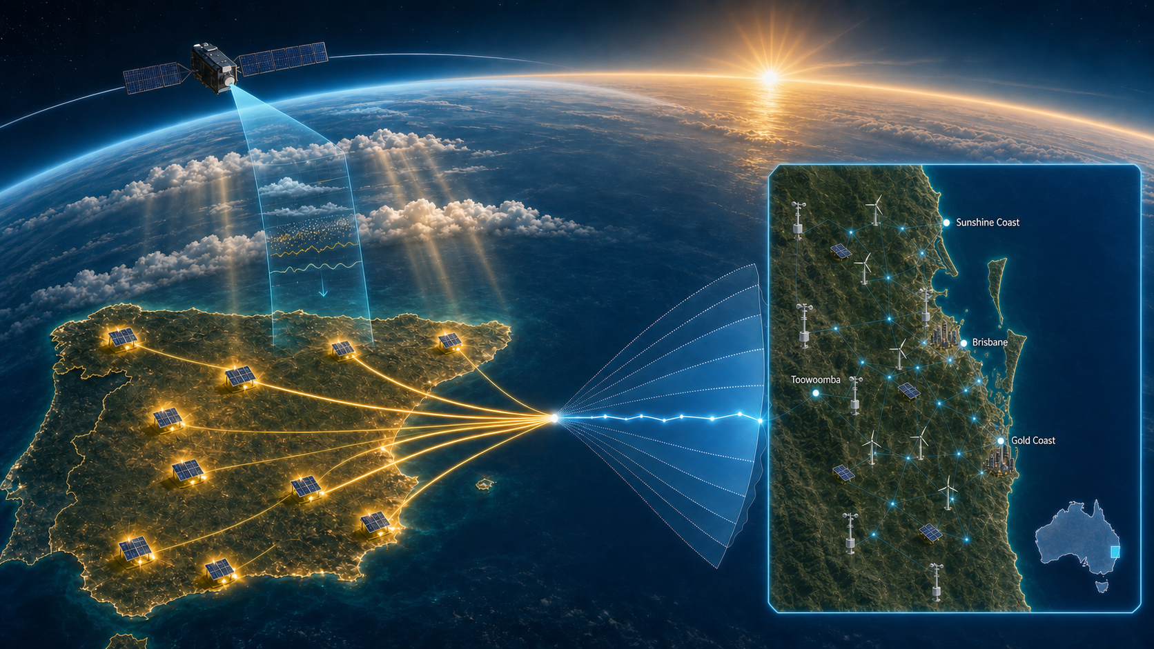
To improve solar forecasting, we replaced the Kaggle weather data with data from the Copernicus Atmosphere Monitoring Service (CAMS), accessed through the Atmosphere Data Store. CAMS provides global atmospheric and solar-radiation products, including the CAMS solar radiation time-series. For solar power, the most useful variable is global horizontal irradiation (GHI), which measures solar energy received at ground level and already responds to cloud cover and atmospheric conditions.

 

Choosing Solar-Plant Locations

Instead of querying CAMS for arbitrary cities, we selected major solar plants that were operational during the 2015-2018 period. We focused on nine of the largest plants with reliable capacity and location information, including Solaben, Solnova, Andasol, Manchasol, Valle, Helioenergy, Solacor, and Aste. These sites represented about 16.6% of Spain's total solar capacity at the time, enough to give us a more physically relevant feature set while keeping the data volume manageable.

 

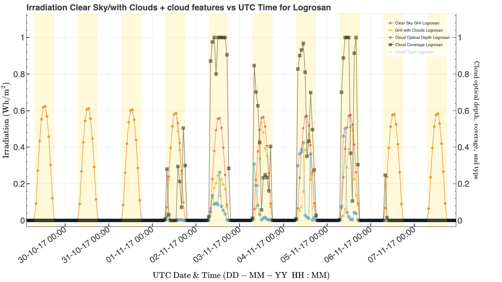
For each location, we requested CAMS data at one-minute cadence and then cleaned and resampled it to hourly resolution to match the Kaggle power data. GHI and clear-sky GHI were summed over each hour, while cloud coverage, optical depth, and snow probability were averaged. Cloud columns required extra care because night-time values were missing; these were filled in a way that avoided unrealistic jumps at sunrise and sunset.

 

CAMS features for the Solaben solar power station near Logrosan. GHI (red line and stars) decreases relative to clear-sky GHI (gold line and triangles) when cloud coverage (black line and squares) and optical depth (blue line and circles) increase, making it a physically meaningful solar forecasting feature.

 

Nationalising CAMS Features

The target solar generation is national, while CAMS features are location-specific. To bridge that gap, we weighted each CAMS location by the solar capacity of the corresponding plant and aggregated across the nine sites. We also engineered additional weighted features: the GHI-to-clear-sky ratio, GHI multiplied by cloud coverage, and GHI multiplied by optical depth. These were designed to help LightGBM capture both irradiance and cloud-related attenuation.

 

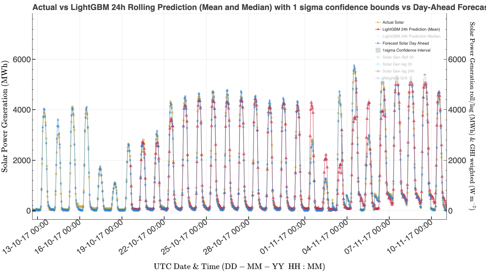
We then trained LightGBM models using the same general strategy as before: a 70/30 split, walk-forward validation, and rolling 24-hour forecasts. The CAMS-based solar model improved over the LightGBM model built only from the Kaggle city-weather features, but the gain was modest. The full-test R² improved from about 0.840 to 0.873, and the rolling 24-hour forecast improved from about 0.860 to 0.886.

 

Rolling 24-hour LightGBM solar forecast using CAMS features with the same plotting colours and symbols as previously used. The model improves modestly but still struggles with some daytime peaks.

 

How Do These Models Compare with the TSO?

The Spanish TSO forecasts still outperform our models for solar, wind, and load. That is not surprising. Operational forecasts have access to information that this dataset does not: plant capacities across the full grid, plant-level telemetry, power curves, detailed weather forecasts near generation assets, and physical/statistical hybrid models. Published descriptions of TSO load forecasting also point to seasonal regression-ARIMA models with weather and holiday effects, while wind and solar systems rely much more directly on plant-level and weather-forecast information.

 

Our results therefore should not be read as a failure of machine learning. They show the importance of problem framing and data relevance. A national model built from five city weather stations is not equivalent to an operational plant-aware forecasting system.

 

Conclusions

This project compared two modelling approaches for Spain's electricity data: ARIMAX and LightGBM. LightGBM outperformed ARIMAX for solar and wind generation, while ARIMAX was stronger for total load and price in this particular setup. The TSO forecasts remained far ahead for solar, wind, and load. The one exception was price, where our ARIMAX price model performed better than the provided price forecast in the experiment, though this result deserves further investigation.

 

The biggest lesson is that feature quality matters more than model complexity. For solar, adding CAMS GHI and cloud information at solar-plant locations improved the LightGBM forecast. For wind, the city-level weather features were too weakly connected to wind-farm conditions. For price, important market drivers were missing entirely.

 

Future Work

The next step is to move from national-scale Spain forecasts to a more local and better-instrumented region. A natural follow-up is southeastern Queensland, where the Australian Energy Market Operator provides energy generation and load data, and the Bureau of Meteorology provides weather observations and forecasts. A smaller region would make it easier to match weather observations to generation assets and load centres.

 

I am also interested in a probabilistic approach. Solar forecasting is inherently uncertain because future cloud cover, GHI, atmospheric opacity, and temperature are uncertain. Deterministic models such as SARIMAX and LightGBM can be very useful, but they do not naturally provide well-calibrated uncertainties. A Bayesian model such as PyMC-BART could incorporate uncertainty in weather forecasts and produce a predictive distribution rather than a single point estimate. That would be closer to what decision-makers need in practice: not just "what will solar generation be?", but "what is the expected generation and how uncertain is it?"

 

Code and notebooks: the project notebooks and supporting code are available on the GitHub repository.

 

Further reading: For background on operational forecasting approaches, see Caro, Juan, and Nouhitehrani (2023), SIPREOLICO, and the eSIOS documentation.

 

 

< Previous Post   |   Data Science Home Page ⌂