Using Machine Learning to Forecast Energy in Spain

Conceptual overview of the LightGBM forecasting workflow. Engineered weather, time, rolling, and lagged features for solar generation, wind generation, total load, and price are passed through an ensemble of boosted decision trees to produce forecasts and uncertainty intervals. Image was generated using AI.

 

Why Try LightGBM?

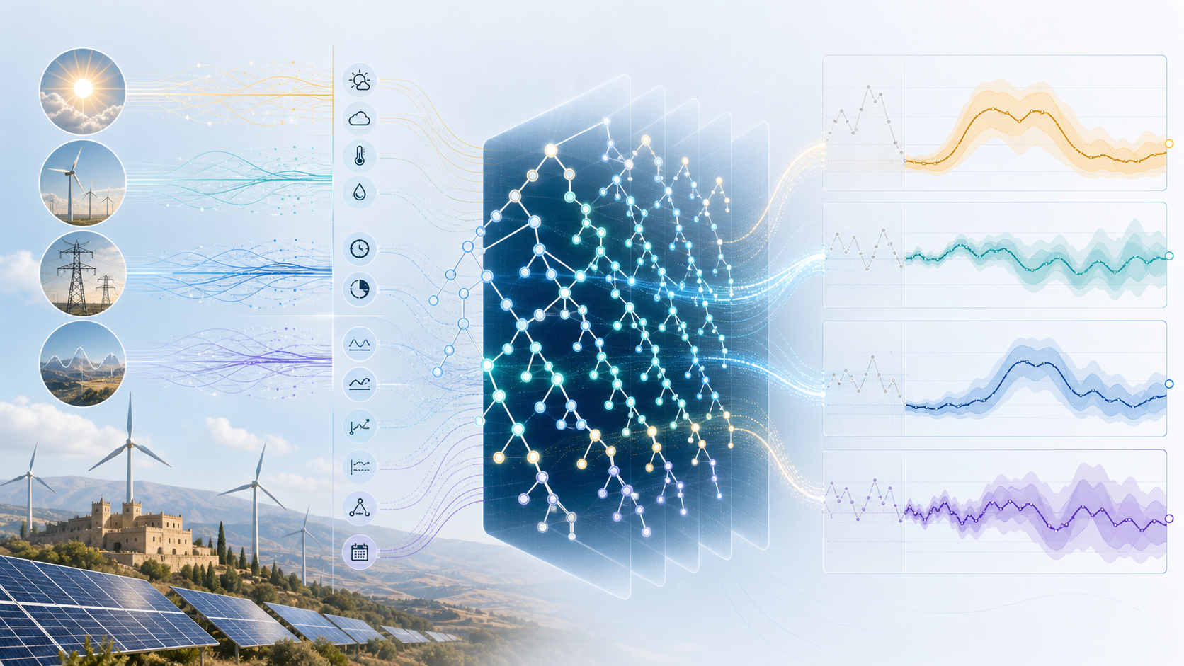
After the ARIMAX baseline, we moved to LightGBM, a gradient-boosted decision-tree model developed by Microsoft Research. Gradient boosting is well suited to tabular datasets with nonlinear relationships, feature interactions, and heterogeneous inputs. LightGBM is also fast and memory efficient, which mattered because this project was developed on a 2018 MacBook Pro rather than a high-performance compute system.

 

The first LightGBM models used the same cleaned and engineered Kaggle-derived features as the ARIMAX models: weighted weather features, solar/time features, rolling averages, lags, holiday flags, and cyclical encodings. We trained a mean regression model and also trained quantile models to estimate P16, P50, and P84 predictions, providing a useful 1σ style prediction band.

 

Solar Generation: A Clear Improvement over ARIMAX

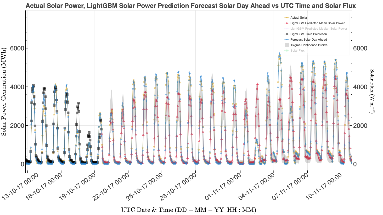
For solar generation, LightGBM performed much better than ARIMAX. The first LightGBM solar model achieved an R² of about 0.84 across the testing period, compared with roughly 0.70 for the best ARIMAX solar model. The day-ahead TSO forecast still performed far better, with an R² near 0.98, but LightGBM captured the broad daily solar generation cycle and responded better to weather and time features.

 

The main weakness remained the daytime peak. The model often predicted the overall cycle well, but generally underestimated the peak generation values. This is important because the peak is often the most operationally relevant part of solar power generation.

 

LightGBM solar generation forecast (represented by the red line triangles) with actual solar generation (given by the gold line and stars), training predictions (black line and squares), the TSO day-ahead forecast (blue line and diamonds), and the P16-P84 prediction band (gray shaded region). LightGBM improves substantially over ARIMAX but still struggles with peak solar output.

 

Walk-Forward Validation

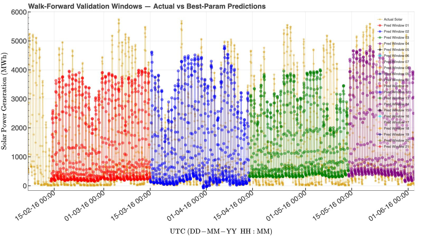
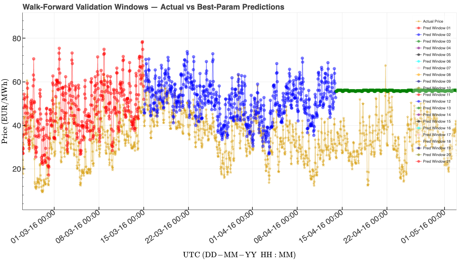
A single 70/30 split is useful, but time-series models can behave differently across seasons and years. To test stability, we used walk-forward validation. The model was trained on a fixed window of past observations, validated on a 30-day window, and then the training and validation windows were advanced forward. This simulates how a model might be evaluated over time without randomly shuffling the data.

 

The walk-forward solar forecasts showed that performance changed somewhat from window to window, but the model was generally stable. The best overall LightGBM solar model from this process achieved an R² close to the first 70/30 model.

 

LightGBM solar walk-forward validation over multiple 30-day windows. This view is useful for checking whether model performance changes over time.

 

A Fairer Comparison: Rolling 24-Hour Forecasts

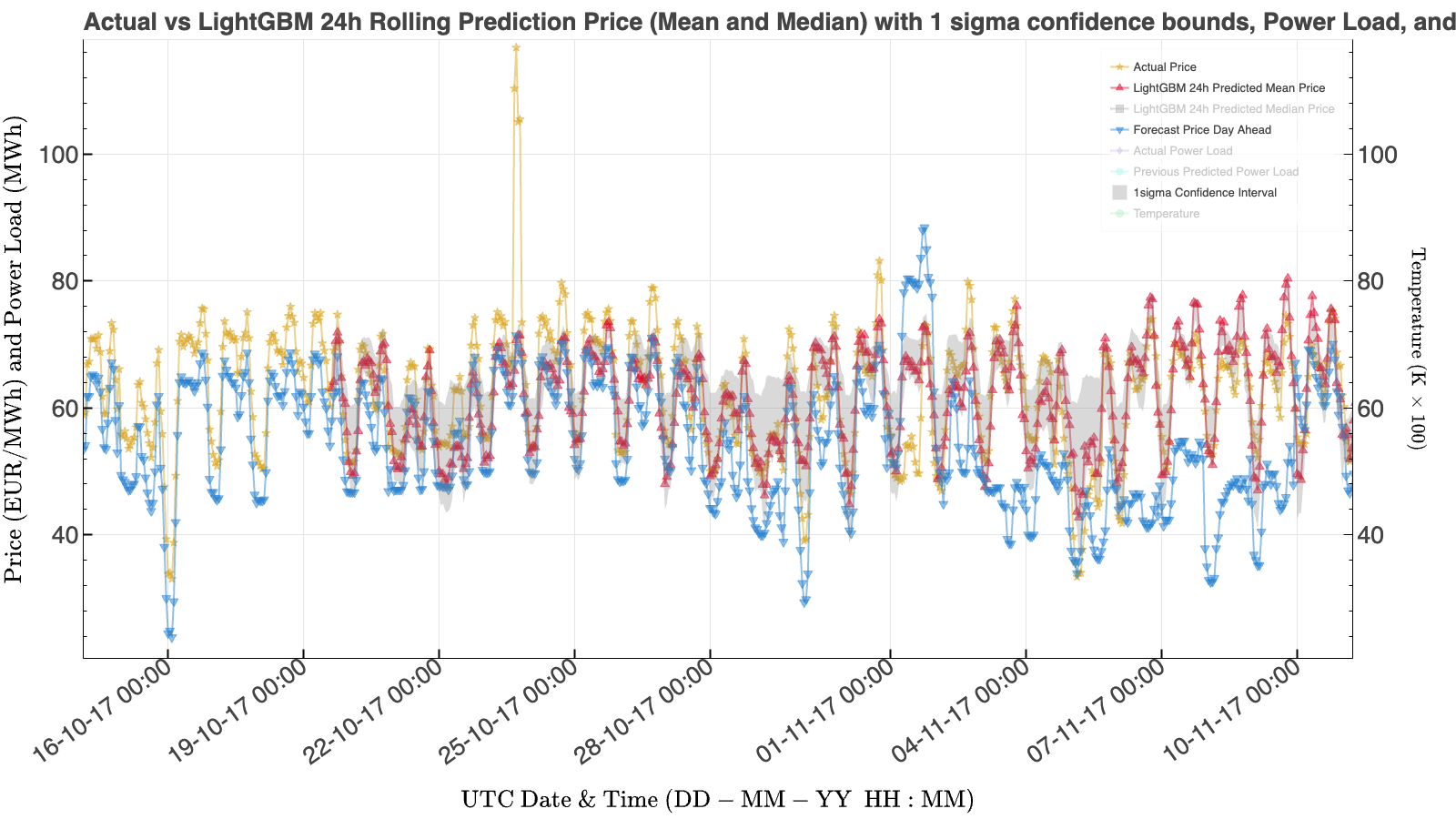
One caveat with the first 70/30 split is that it asks the model to predict over a very long test interval - roughly 14.5 months. The TSO forecast columns, in contrast, are 24-hour forecasts. To make a fairer comparison, we trained on the first 70% of the dataset, predicted the next 24 hours, then advanced by one day, retrained with the newly available data, and predicted the next 24 hours. Repeating this process produced a full test-period sequence of daily forecasts.

 

This improved the LightGBM solar result only slightly, from an R² of about 0.84 to about 0.86. At first that may seem surprising, because 24-hour forecasts should be much easier than 14.5-month forecasts. The explanation is that both forecast models used actual observed weather as input features. A real operational forecast would need weather forecasts, so these forecasts are still optimistic and would likely perform worse (but with the 24-hour forecast less impacted).

 

Wind, Load, and Price with LightGBM

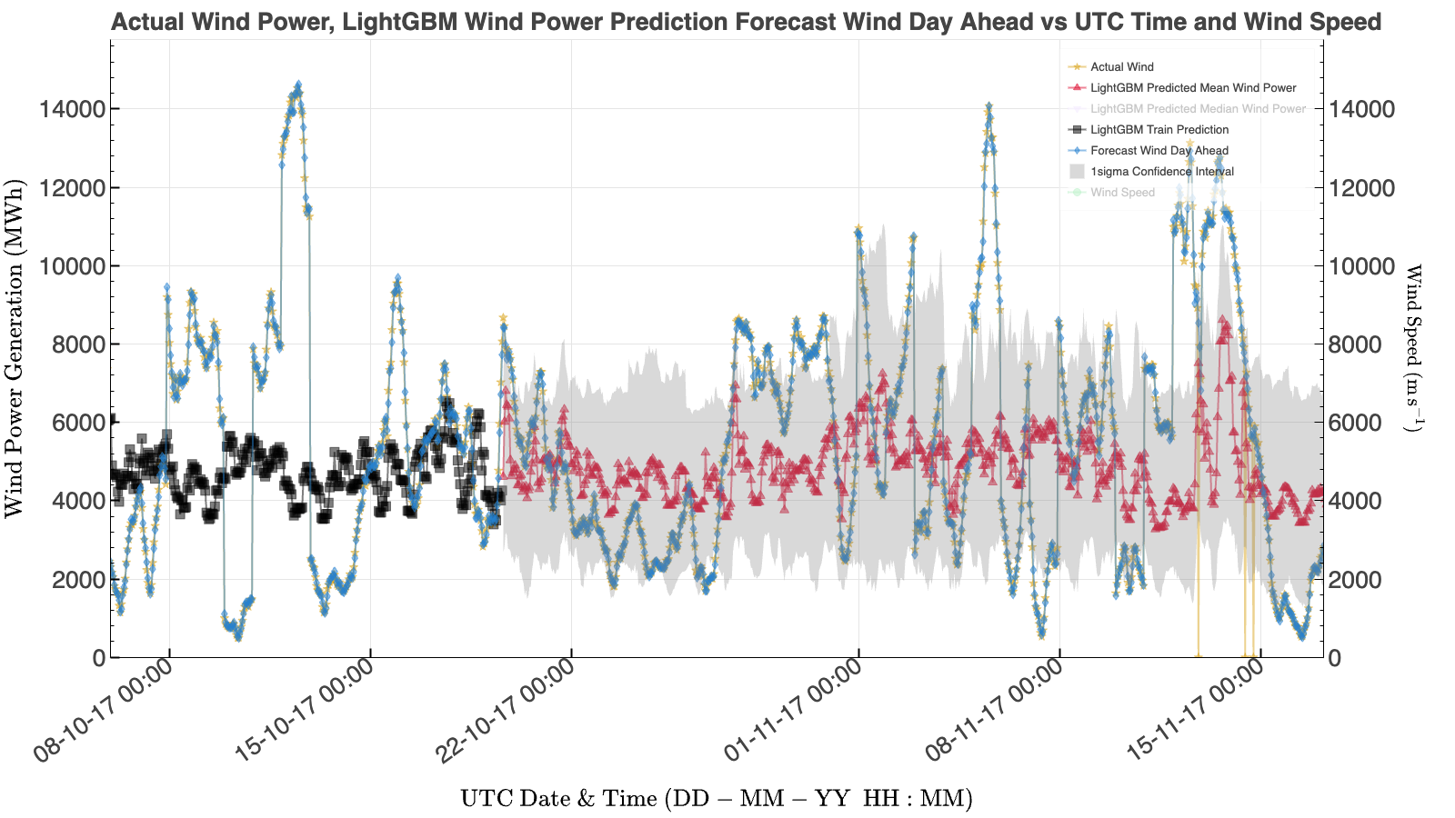
Wind generation remained difficult. LightGBM improved slightly over ARIMAX, but the R² stayed low and the TSO forecast remained vastly better. Again, this points to feature limitations: city-level wind speed is a poor proxy for wind conditions at wind farms across Spain.

 

LightGBM wind generation forecast using the same plotting symbols and colours as used in previous figures. The model struggles on both the training and testing intervals, consistent with weak feature-target relationships for wind generation.

 

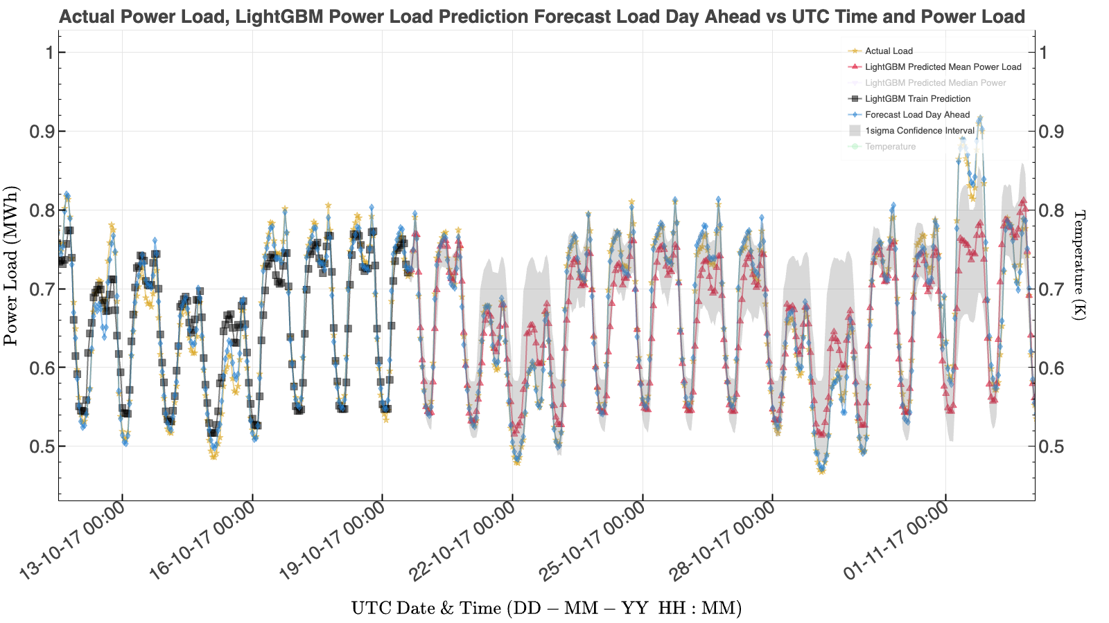
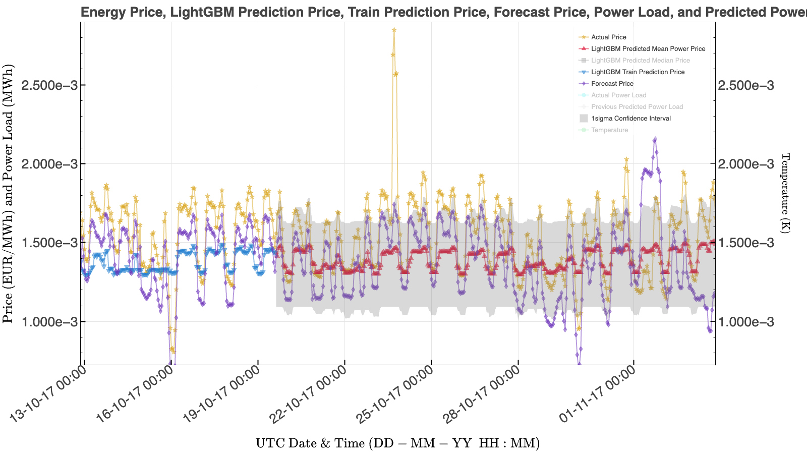
For total load and price, LightGBM was not uniformly better than ARIMAX. Total load forecasting with LightGBM performed worse than ARIMAX and the TSO benchmark. Price forecasting was even more challenging, with large variations across walk-forward windows. The daily rolling price forecast improved over the long-horizon test forecast, but it was still not strong enough to be considered reliable.

 

Left: LightGBM total load forecast using the same plotting symbols and colours as used in previous figures. It captures some daily structure but underperforms the TSO forecast and the ARIMAX load model. Right: LightGBM price forecast using the same plotting symbols and colours as used in previous figures. The model struggles to forecast prices, capturing little of the daily structure.

 

Left: LightGBM price walk-forward validation. The model performance varies considerably between validation windows. Right: LightGBM daily price forecast using the same plotting symbols and colours as used previously. The LightGBM daily price forecast provides a significant improvement over the long-horizon test forecast.

 

Interpreting the LightGBM Results

The LightGBM results were a useful reminder that model flexibility is not a magic fix. LightGBM clearly helped for solar generation, where the engineered time and irradiance-related features were informative. It helped only modestly for wind, where the available weather data were not well aligned with the generation sites. It performed poorly for price, where market structure, bidding behaviour, fuel mix, interconnector flows, and other variables not present in the dataset likely matter.

 

Key takeaway: LightGBM is powerful, but the largest performance gains still come from better features and better geographic alignment between weather observations and energy assets.

 

 

< Previous Post   |   Data Science Home Page ⌂   |   Next Post >