Using Machine Learning to Forecast Energy in Spain

Conceptual overview of the Part 2 workflow. Solar and wind generation data are transformed using weather, time, cyclical, rolling, and lagged features before an ARIMAX baseline is compared with Spain's day-ahead TSO forecast. Image was generated using AI.

 

From Cleaned Data to Model-Ready Features

After cleaning the Spain power and weather data, the next challenge was feature engineering. The targets - solar generation, wind generation, total load, and price - are national values, but the weather observations are city-level measurements. To make the features match the national targets, we aggregated weather features across the five cities using population-based weights. This is a reasonable first-order approximation for load forecasting, although it is less physically appropriate for generation, where the locations of solar plants and wind farms matter much more.

 

We also added time features that should help the models learn predictable cycles: month, day of year, day of week, weekend flag, public holidays, sunrise and sunset times, daylight length, and cyclical sine/cosine encodings for the hour of day, day of week, day of year, and month. For solar, we also calculated an approximate solar flux using the Sun's position. Rolling and lagged features were added carefully using shifted values so that each row only had access to the past, avoiding data leakage.

 

Before fitting models, we explored Pearson and Spearman correlations between candidate features and the targets. One surprising result was that city-level cloud cover was only weakly correlated with national solar generation. That was an early clue that the OpenWeather city observations were not geographically well aligned with Spain's solar plants.

 

Why Start with ARIMAX?

SARIMA-style models are a classic baseline for seasonal time series. SARIMAX extends this framework by adding exogenous variables, so it can use weather and time features in addition to the target's own history. We used SARIMAX through the Python statsmodels implementation as an ARIMAX-style baseline.

 

The advantage of ARIMAX is interpretability: it forces us to think about stationarity, differencing, autoregressive lags, moving-average terms, and seasonal structure. The disadvantage is that the model is fundamentally linear in the exogenous regressors and can struggle with nonlinear weather relationships. For solar and wind, those nonlinearities matter.

 

Solar Generation with ARIMAX

We began with solar generation because it has the clearest physical cycle. A daily seasonal period of 24 hours is the obvious starting point, so our first serious model used an ARIMAX order of (1, 0, 1) and a seasonal order of (1, 0, 1, 24). We also tested stationarity with the Augmented Dickey-Fuller and KPSS tests, which suggested that first-order differencing may be needed.

 

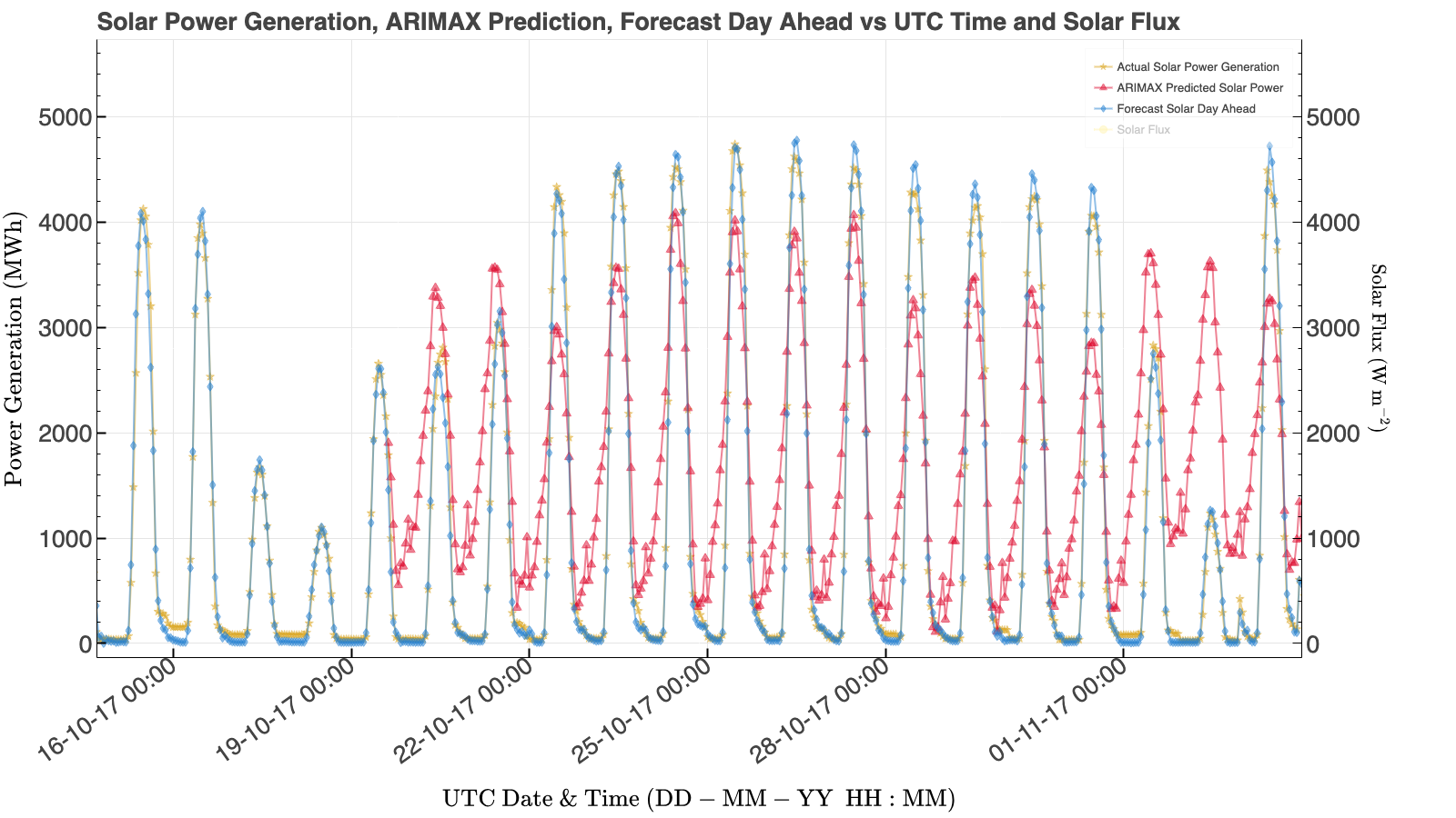
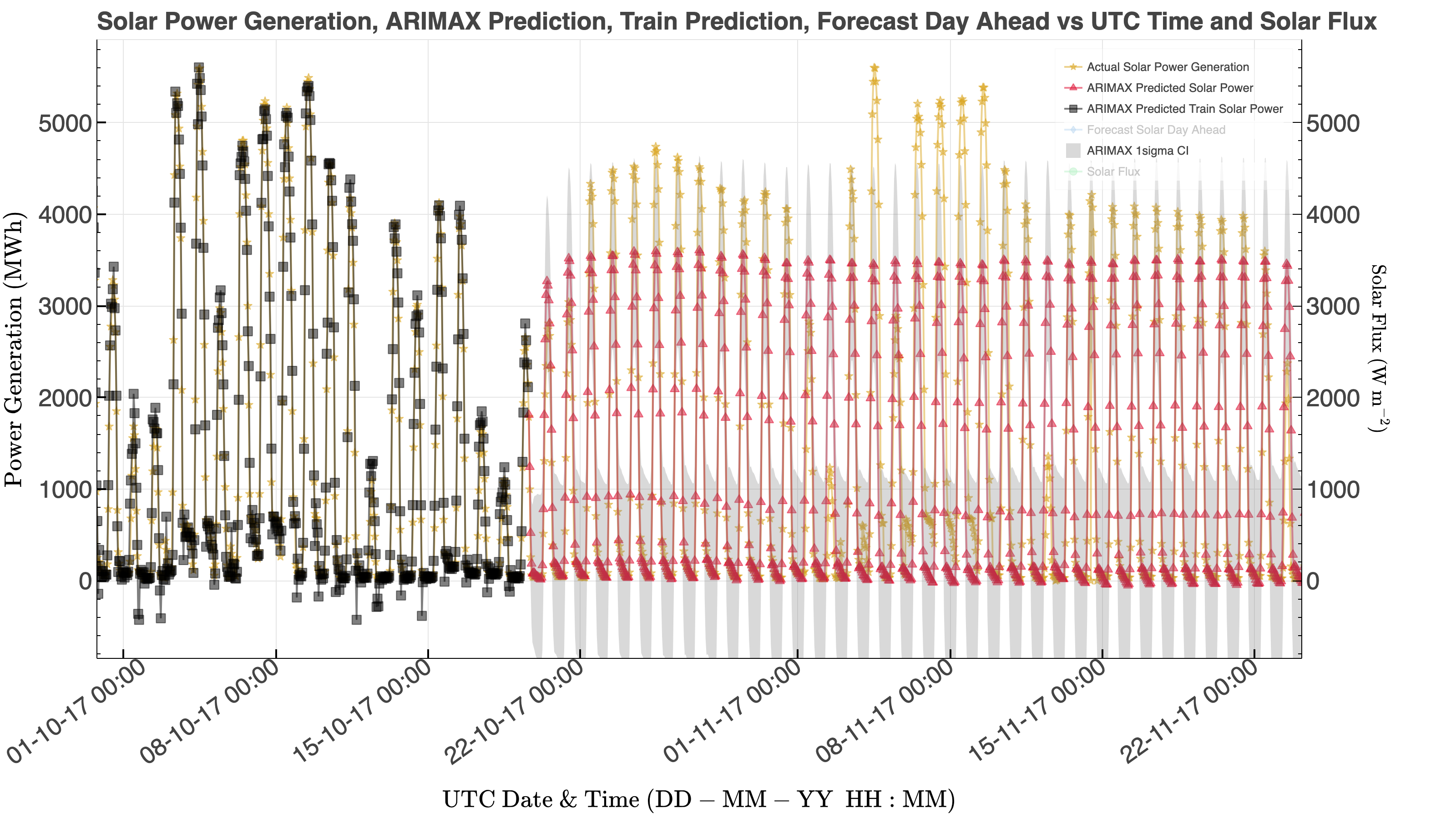
The baseline ARIMAX model performed poorly. It struggled with both nighttime minima and daytime peaks, and it was dramatically worse than Spain's day-ahead solar forecast. A grid search over ARIMAX and seasonal ARIMAX orders improved the R² fitting statistic value, but much of the gain came from better nighttime predictions rather than more accurate daytime peaks. The model still failed to react strongly to weather-driven changes in peak solar output.

 

Left: Baseline ARIMAX solar forecast using order (1, 0, 1) and seasonal order (1, 0, 1, 24) shown as the red line and triangles. The model struggles compared with the day-ahead benchmark (blue line and diamonds). The observed (actual) solar generation is given as the gold line and stars. Right: Solar forecast after grid-searching ARIMAX orders (using the same plotting symbols and colours as before) with the training model given as the black line and squares. The fit improves, but the daytime peak is still too rigid across the test period.

 

Wind Generation and Seasonality

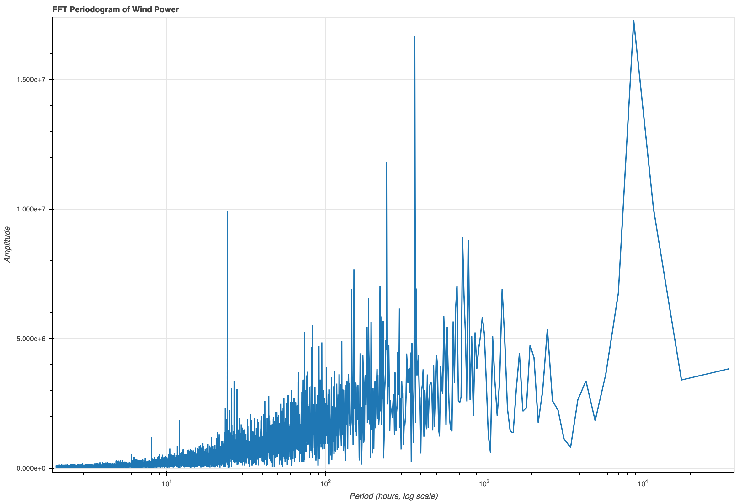
Wind forecasting was even more difficult. Seasonal decomposition suggested that a 24-hour period gave the smallest residuals among the periods tested, but the wind signal was much noisier than solar. To check this further, we used a fast Fourier transform and looked at the strongest periodogram peaks. The most noticeable periods were near 24 hours, roughly 244 hours, and roughly 366 hours. We kept the 24-hour seasonal period because it appeared most significant relative to the local noise floor.

 

Wind generation periodogram produced from a fast Fourier transform. The most prominent peaks are near 24 hours, 244 hours, and 366 hours, but we went with the 24-hour signal in our SARIMAX model as it was the most useful period in practice.

 

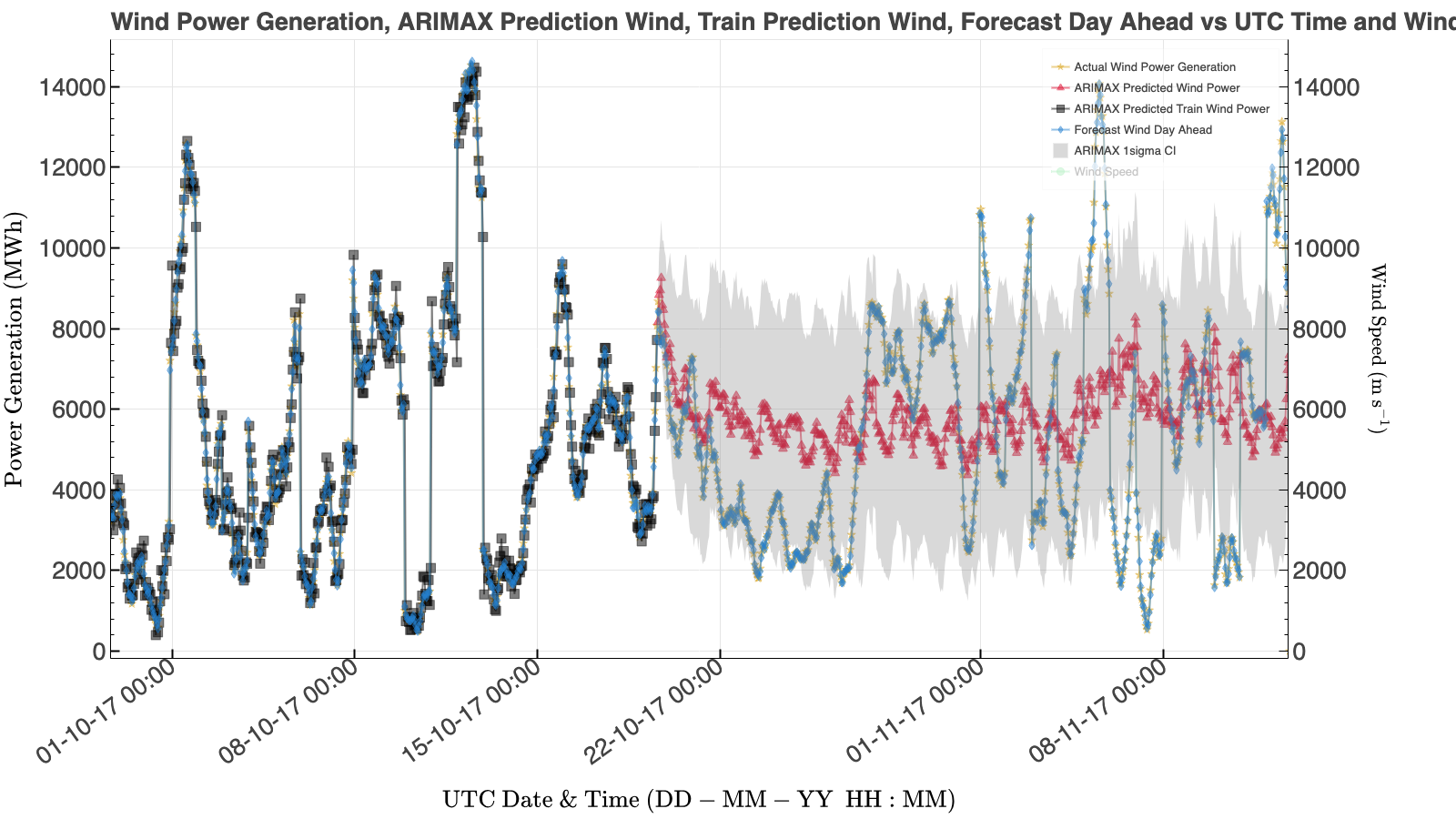
Even with tuned ARIMAX orders, wind forecasts remained poor. The likely reason is not simply model choice; it is feature relevance. Wind speed measured in five large cities is unlikely to capture conditions at the wind farms that produce national wind generation. This geographic mismatch limits the model before the algorithm even has a chance.

 

ARIMAX wind forecast, given as the red line and triangles. The model fits the training data (training model shown as the black line and squares) better than the forecast horizon and remains far behind the operational wind forecast (blue line and diamonds). The actual observed wind power generation is given by the gold line and stars.

 

Load and Price Forecasting

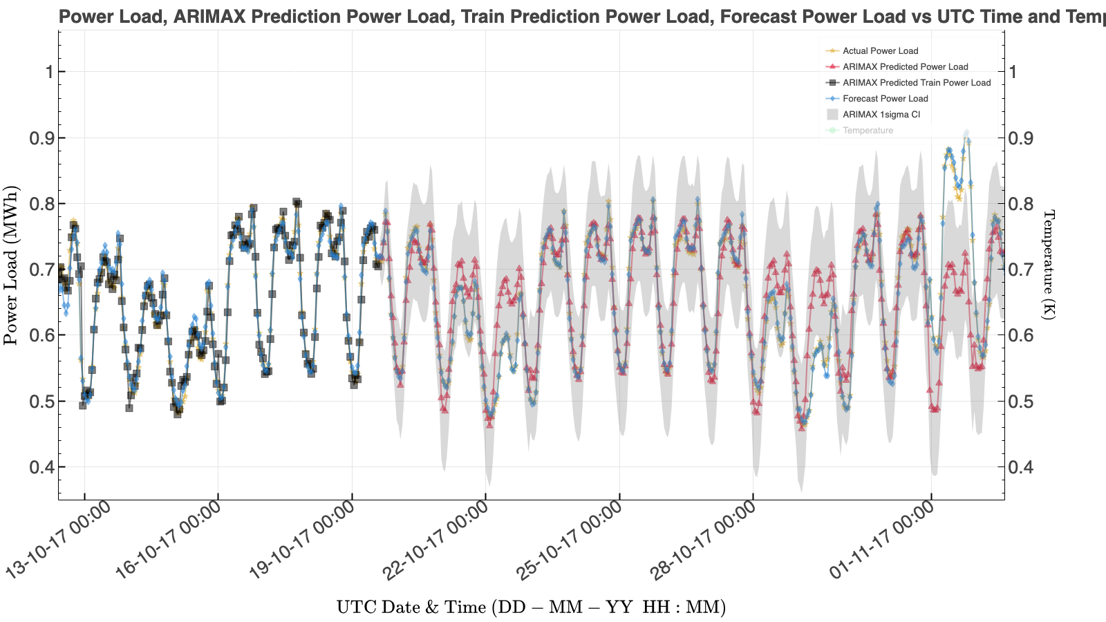
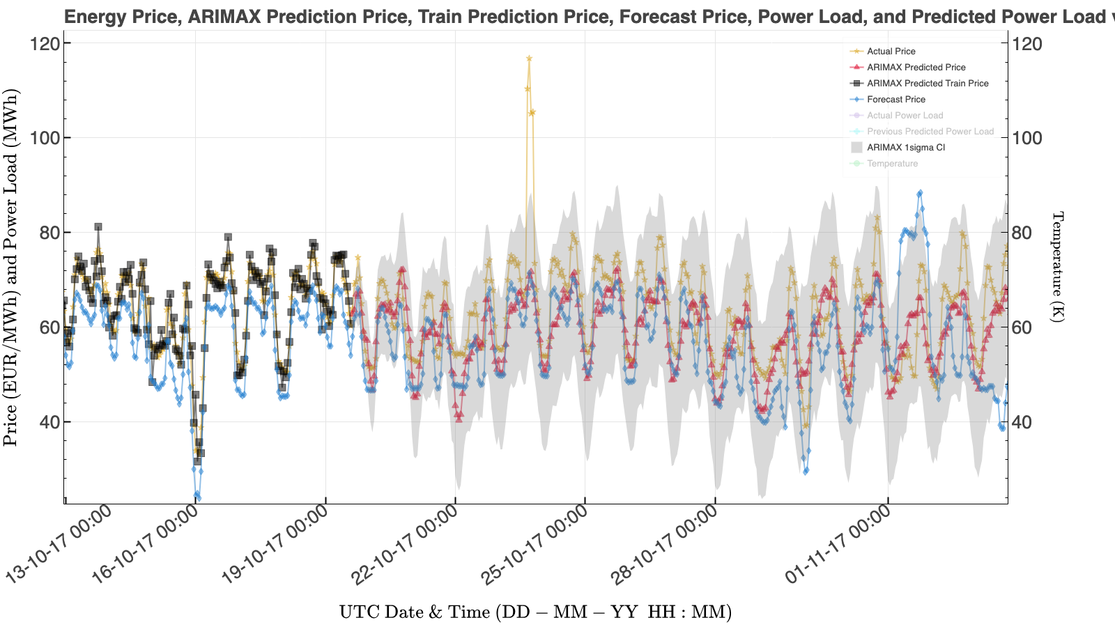
Total load behaved more like a traditional demand forecasting problem. It has a strong daily rhythm, weekly structure, holiday effects, and correlations with temperature and humidity. The ARIMAX load model performed reasonably well, although it still lagged the TSO forecast. Interestingly, the ARIMAX price model did better relative to the published price forecast than our generation models did. Since price depends strongly on load, we forecast load first and then used the predicted load as an input feature for the price model to avoid leakage.

 

Left: ARIMAX forecast of total load as shown as the red line and triangles. The model captures the broad daily cycle but misses some higher and lower load events. Right: ARIMAX price forecast, also given as the red line and triangles. Price forecasting is noisy, but this model performed better than the published price forecast in this experiment.

 

What We Learned from the Baseline

ARIMAX was a useful baseline, but it exposed the limits of linear time-series models for this problem. Solar and wind forecasts were especially constrained by the mismatch between national generation and city-level weather features. Load was more tractable, and price was sensitive to how load was handled. In the next post, we switch to LightGBM, which is better suited to nonlinear interactions and more flexible feature relationships.

 

Key takeaway: A model can be statistically sophisticated and still fail if the feature set does not represent the physical system well.

 

 

< Previous Post   |   Data Science Home Page ⌂   |   Next Post >